
|
| Figure 1. Color scale editor in Data Explorer. |
Color is an important dimension in visualizations. A well-chosen encoding can make features and patterns in data easy to find and analyze. There are many possible ways of coloring the values of a single continuous variable, but they all involve the mapping of a set of values to a color scale, an ordered arrangement of colors. Color scales are also called color ramps. Some common color scales are (1) a gradient from black to white (a greyscale ramp) and (2) a rainbow-like scale that passes through blue, cyan, green, yellow, and red.
Choosing a good color scale is an important step in crafting an effective visualization. Users typically apply a predefined color scale or create their own with a color scale editor. Users of the IBM Data Explorer visualization tool, for example, can create a new color scale using a flexible color scale editor (see Figure 1), or choose a predefined color scale with the guidance of the PRAVDAColor module, which offers suggestions based on the characteristics of their data and their expressed visualization goals.
Figure 1. Color scale editor in Data Explorer.
Although there may be differences in detail, such as the colors employed, the overall design of color scales for displaying a single continuous variable is predictable. It usually consists of some linear progression of colors, scaled such that the first color corresponds to the minimum value and the last color to the maximum value in the range of the variable. Although sufficient for most cases, it is not too hard to imagine real data sets for which a single color scale of this basic design would be inadequate. For example, it would be a poor match for a data set in which most values are clustered in a narrow range even though the minimum and the maximum are widely separated (by, say, many orders of a magnitude). Because the available colors must represent the entire range of values, few colors would be devoted to the relatively narrow cluster of values, and thus detail would be lost. If such detail is important, then something must be done to bring it out. Obvious ways are by filtering the data and by narrowing the view upon the data. These methods are straightforward to implement and often very effective. This paper proposes an additional method which may be useful in similar situations. The basic idea is to distort the color scale such that more colors are applied to the region of interest and fewer elsewhere.
Nonlinear color scales are a direct application of nonlinear magnification techniques. Like other Focus+Context techniques, the main goal of nonlinear color scales is to make the most of a limited resource--the set of distinguishable shades of colors in this case. By alloting more colors to areas of interest and fewer colors to all other areas, color can become a tool for interactively exploring fine detail. There are other well-established and complementary methods for exploring data, such as filtering and aggregating, but a technique based on color has the advantage of making use of the power and immediacy of our visual system.
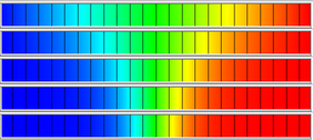
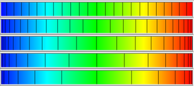
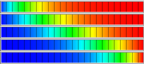
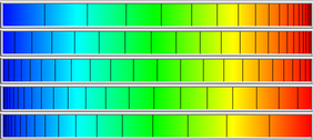
There are two equivalent formulations of this technique. The technique can be implemented by distorting either the color space or the value space. Figures 2 and 3 show how these formulations differ conceptually. Their difference in appearance is only superficial, however, as the effect is the same. In each figure, the left column shows distortion in the color space, and the right shows distortion in the value space. The vertical lines mark off equal intervals of values, and each column shows five snapshots of a color scale undergoing some change. In Figure 2, the successive rows show an increase in magnification, with the bottom row showing the highest level. In Figure 3, the rows show a left-to-right movement of the focus of magnification.
Although these figures use the hot-to-cold color ramp, the technique itself is applicable to any color scheme, though some will be better suited than others. In actual practice, the color scheme will most likely involve a change in luminance or saturation, rather than hue, as a change in hue is considered ill-suited to representing continuous variables by some.
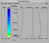
A nonlinear color scale is no more than a particular arrangement of colors. Thus, in principle, it requires no more supporting machinery than a color scale editor. For example, one could imagine adapting the powerful color gradient editor (see Figure 4) in GIMP for this purpose, as it already supports nonlinear interpolation between colors. Even a tool as powerful as this, however, would soon become tedious to use during interactive exploration, if the user has to manually piece together each of possibly many color scales. For this technique to be maximally useful, there must be direct high-level support for creating nonlinear color scales. The ideal mechanism would automatically generate them based on a few intuitive parameters supplied by the user. We present one possible implementation, in which the parameters are magnification level and focus location.

Figure 4. Color gradient editor in GIMP.
Our approach is to map values to colors using a continuous nonlinear function. We describe two such functions, but their choice is largely arbitrary, as the technique of nonlinear color scales is not about the use of any particular function. Any strictly-increasing function with parameters for adjusting the magnification and focus could be used instead. For the purposes of discussion, we assume that the value space has been mapped into the closed interval [0, 1]. We further assume that there is a mapping between the closed interval [0, 1] to some user-chosen color scheme (some sequence of colors). Thus, the central task is to map [0, 1] onto itself with nonlinear distortion.
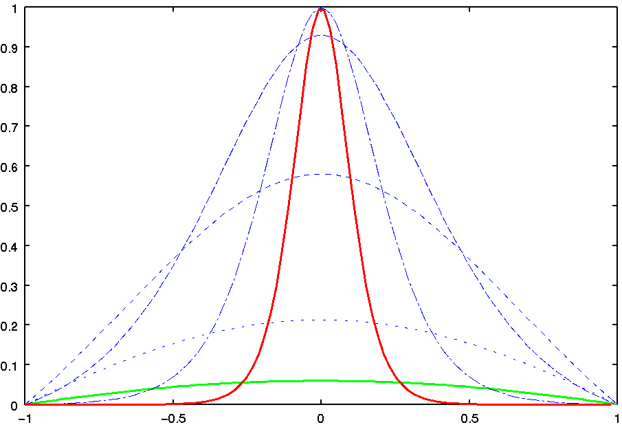
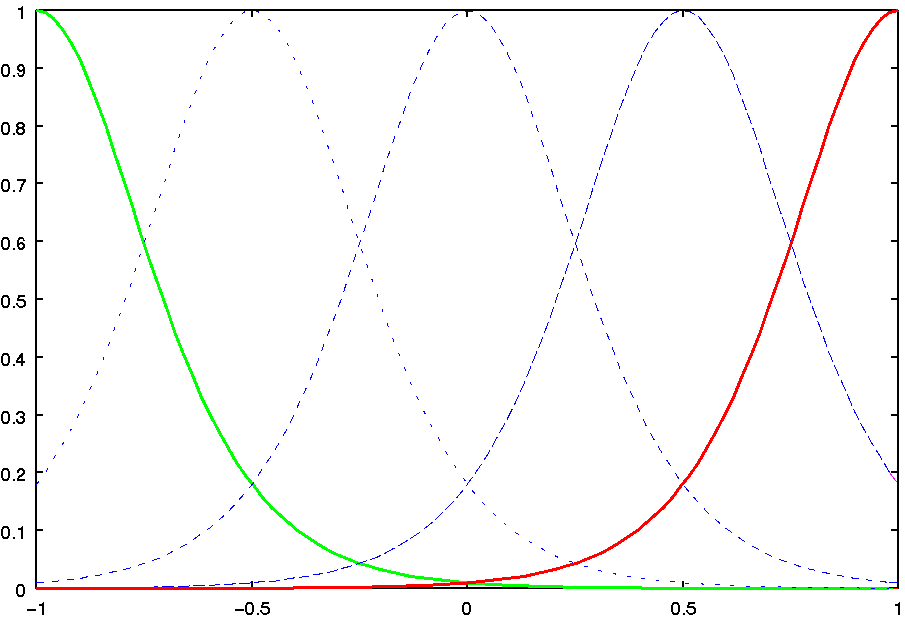
Leung and Apperley introduced the distinction between magnification and transformation functions. The former is the derivative of the latter, and expresses the desired degree of magnification at each point in the domain. Peaks correspond to areas of high magnification, and troughs to areas of low magnification. This function corresponds more closely to our intuitive idea of the distortion process. Nevertheless, it is the transformation function that actually performs the distortion. Figures 5 and 6 show the common form of our distortion functions. Figure 5 shows how changing the level of magnification affects the shape of the magnification and transformation functions. Figure 6 shows the effect of moving the focus location. In both figures, green and red lines represent the functions under the starting and ending values, respectively, of the parameter. The blue lines represent intermediate stages.
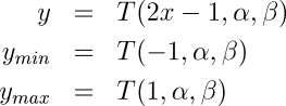
Given a transformation function T(x, alpha, beta), where x (in [0,1]) is the coordinate to transform, alpha specifies focus location, and beta specifies magnification level, we compute y' (in [0,1]) as follows:
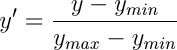
where
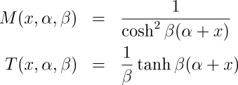
The following is a pair of magnification and transformation functions which could be used for this purpose (alpha should vary between -1 and 1, and a good range for beta is [0.5, 5.5]):
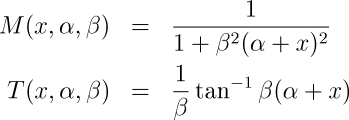
Another pair, similar in shape to the first but with a gentler drop-off in magnification, is the following (the above ranges for alpha and beta also work here):
The above formulas are meant to be clear rather than maximally efficient. One improvement would be the elimination of the scaling by 1/beta in the transformation functions, but doubtless there are others, including the use of piecewise approximations.
The above transformation functions suffer from a minor defect. Slope directly corresponds to magnification level in the graphs of transformation functions. However, Figure 6(b) clearly shows that slope changes as the focus moves to either end of the range with these transformation functions. This defect results from our simplistic scaling of the range to [0,1]. We would like to correct this in the future.
We would also like to try other transformation functions. Ones based on raising x to a variable power seem promising. Another worth trying is the transformation function of the Graphical Fisheye View.
Nonlinear Magnification:
Color scales:
Color science:
Organizations: